GDP Analysis

Background

Gross Domestic Product (GDP) measures the market value of all the final goods and services produced in a specific time period. According to Wikipedia, GDP (Y) can be written as below:

Y = C + I + G + (X − M)

C (consumption)：Consisting of private expenditures in the economy, named as Household Expenditure in our data
I (investment): Business investment, named as Gross Capital Formation in our data
G (government spending): Sum of government expenditure, named Government expenditure in out data
X (exports): Gross exports, same name in our data
M (imports): Gross imports, same name in our data
X - M (net exports): Net exports, not given in data but easy to calculate with code

In this analysis, we look at GDP and GDP components from mature and emerging markets (3 selected countries in each) between 1970 to 2017, estimated by United Nations’ National Accounts Main Aggregates Database. You can download the data here .

Load packages

library(readxl) # Read Excel
library(here) # Get local repository 
library(skimr) # Skim a dataframe
library(countrycode) # Map country name to region, continent, currency .etc
library(scales) # Change scales in ggplot
library(patchwork)
library(tidyverse)  # Load ggplot2, dplyr, and all the other tidyverse packages

Load the data

UN_GDP_data  <-  read_excel(here::here("data", "Download-GDPconstant-USD-countries.xls"), # Excel filename
                sheet="Download-GDPconstant-USD-countr", # Sheet name
                skip=2) # Number of rows to skip

Data Manipulation

First, we have a look at our data. It has 3685 rows, and 51 variables. We can see it has indicator name in a column and each year’s value in its own column.

head(UN_GDP_data)

## # A tibble: 6 x 51
##   CountryID Country IndicatorName `1970` `1971` `1972` `1973` `1974` `1975`
##       <dbl> <chr>   <chr>          <dbl>  <dbl>  <dbl>  <dbl>  <dbl>  <dbl>
## 1         4 Afghan… Final consum… 5.56e9 5.33e9 5.20e9 5.75e9 6.15e9 6.32e9
## 2         4 Afghan… Household co… 5.07e9 4.84e9 4.70e9 5.21e9 5.59e9 5.65e9
## 3         4 Afghan… General gove… 3.72e8 3.82e8 4.02e8 4.21e8 4.31e8 5.98e8
## 4         4 Afghan… Gross capita… 9.85e8 1.05e9 9.19e8 9.19e8 1.18e9 1.37e9
## 5         4 Afghan… Gross fixed … 9.85e8 1.05e9 9.19e8 9.19e8 1.18e9 1.37e9
## 6         4 Afghan… Exports of g… 1.12e8 1.45e8 1.73e8 2.18e8 3.00e8 3.16e8
## # … with 42 more variables: `1976` <dbl>, `1977` <dbl>, `1978` <dbl>,
## #   `1979` <dbl>, `1980` <dbl>, `1981` <dbl>, `1982` <dbl>, `1983` <dbl>,
## #   `1984` <dbl>, `1985` <dbl>, `1986` <dbl>, `1987` <dbl>, `1988` <dbl>,
## #   `1989` <dbl>, `1990` <dbl>, `1991` <dbl>, `1992` <dbl>, `1993` <dbl>,
## #   `1994` <dbl>, `1995` <dbl>, `1996` <dbl>, `1997` <dbl>, `1998` <dbl>,
## #   `1999` <dbl>, `2000` <dbl>, `2001` <dbl>, `2002` <dbl>, `2003` <dbl>,
## #   `2004` <dbl>, `2005` <dbl>, `2006` <dbl>, `2007` <dbl>, `2008` <dbl>,
## #   `2009` <dbl>, `2010` <dbl>, `2011` <dbl>, `2012` <dbl>, `2013` <dbl>,
## #   `2014` <dbl>, `2015` <dbl>, `2016` <dbl>, `2017` <dbl>

To make our work easier, we reshape this data to a longer form, having all the years in one column, and all the values in one column. We also want to select only GDP and GDP components in the indicators, then show values in billions.

tidy_GDP_data  <-  UN_GDP_data %>%
  
  # reshape data using pivot_longer
  pivot_longer(cols = 4:51, names_to = 'Year', values_to = 'Value') %>% 
  
  # only keep GDP and GDP components
  filter(IndicatorName %in% c('Gross capital formation', 
                    'Exports of goods and services',
                    'Imports of goods and services',
                    'General government final consumption expenditure',
                    'Household consumption expenditure (including Non-profit institutions serving households)',
                    'Gross Domestic Product (GDP)')) %>%
  
  # give indicators into shorters using case_when and mutate
  mutate(IndicatorName = case_when(IndicatorName == 'Gross capital formation' ~ 'Gross capital formation',
                 IndicatorName == 'Exports of goods and services' ~ 'Exports',
                 IndicatorName == 'Imports of goods and services' ~ 'Imports',
                 IndicatorName == 'General government final consumption expenditure' ~ 'Government expenditure',
                 IndicatorName == 'Household consumption expenditure (including Non-profit institutions serving households)' ~ 'Household expenditure',
                 
                 # Given GDP and calculated (by components) GDP are not identical, so we rename it as GDP_given 
                 IndicatorName == 'Gross Domestic Product (GDP)' ~ 'GDP_given'), 
         
         # show values in billions
         Value = Value/1e9,
         
         # map country to region, function fails to match Micronesia, so we add it manually
         Region = countrycode(Country, origin = 'country.name', destination = 'region',
                              custom_match = c("Micronesia (FS of)" = "East Asia & Pacific"))) 

glimpse(tidy_GDP_data)

## Rows: 63,072
## Columns: 6
## $ CountryID     <dbl> 4, 4, 4, 4, 4, 4, 4, 4, 4, 4, 4, 4, 4, 4, 4, 4, 4, 4, …
## $ Country       <chr> "Afghanistan", "Afghanistan", "Afghanistan", "Afghanis…
## $ IndicatorName <chr> "Household expenditure", "Household expenditure", "Hou…
## $ Year          <chr> "1970", "1971", "1972", "1973", "1974", "1975", "1976"…
## $ Value         <dbl> 5.07, 4.84, 4.70, 5.21, 5.59, 5.65, 5.68, 6.15, 6.30, …
## $ Region        <chr> "South Asia", "South Asia", "South Asia", "South Asia"…

Most and least % GDP growth

Lots of things happened during 1970 - 2017, in this chapter we want to see who has seen the most and the least % GDP growth in this period.

To calculate the % growth, it’s easier to go back to the untidy form of dataframe, to have it in a wider shape. I want to practice pivot_longer/pivot_wider functions just learned, but group_by and summarise functions from tidyverse should also work.

GDP_data_start_and_end <- tidy_GDP_data %>% 
  
  filter(Year %in% c(1970, 2017), # the start and end of this period
         IndicatorName == 'GDP_given') %>% # only keep GDP_given in our indicators
  
  pivot_wider(names_from = Year, values_from = Value) %>% 
  
  mutate(GrowthRate = `2017`/`1970` - 1)

head(GDP_data_start_and_end,3)

## # A tibble: 3 x 7
##   CountryID Country    IndicatorName Region             `1970` `2017` GrowthRate
##       <dbl> <chr>      <chr>         <chr>               <dbl>  <dbl>      <dbl>
## 1         4 Afghanist… GDP_given     South Asia          10.7    22.2       1.07
## 2         8 Albania    GDP_given     Europe & Central …   3.63   14.0       2.85
## 3        12 Algeria    GDP_given     Middle East & Nor…  39.9   199.        3.98

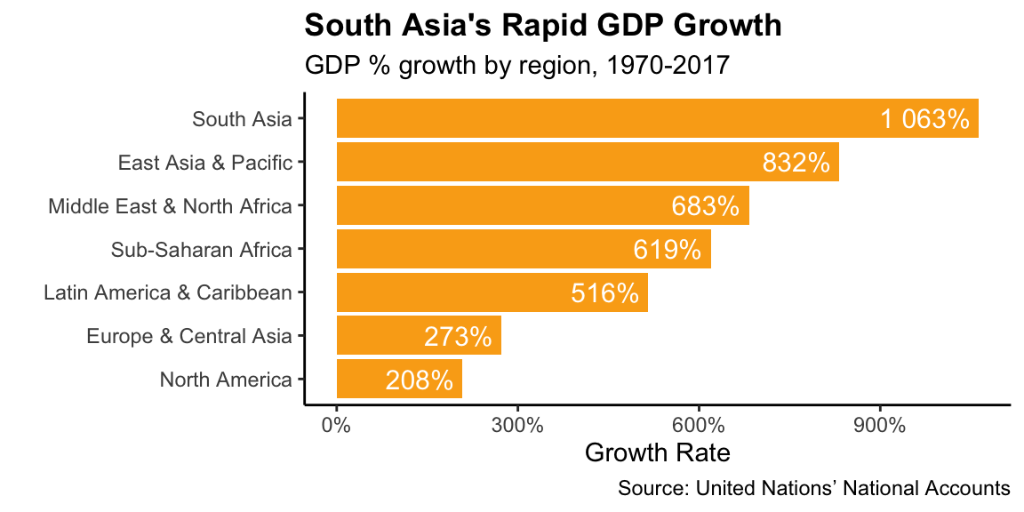
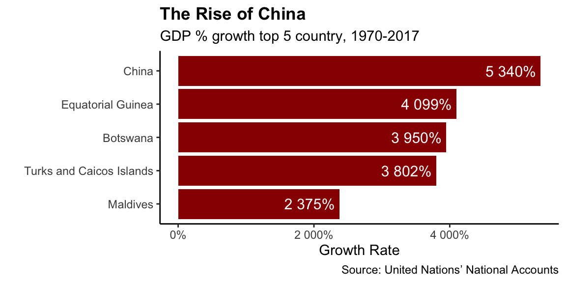
Now, let’s see the ranking of GDP growth by visualization. It turns out South Asia is emerging quickly during this time, while North America has relatively lower % growth in GDP. Still, South Asia is the last but one region in GDP value by 2017. Country-wise, China and Equatorial Guinea have seen the most and second most GDP % growth from 1970 to 2017.

GDP Components Proportion

We then look at GDP components proportion over years. We selected 3 countries from emerging markets and 3 from mature markets to draw comparison. We reshape data again to suit our specific need.

GDP_breakdown <- tidy_GDP_data %>% 
  pivot_wider(names_from = IndicatorName, values_from = Value) %>% 
  mutate(`Net Exports` = `Exports` - `Imports`,
         `GDP_calculated` = `Government expenditure` + 
           `Gross capital formation` +
           `Household expenditure` +
           `Net Exports`)

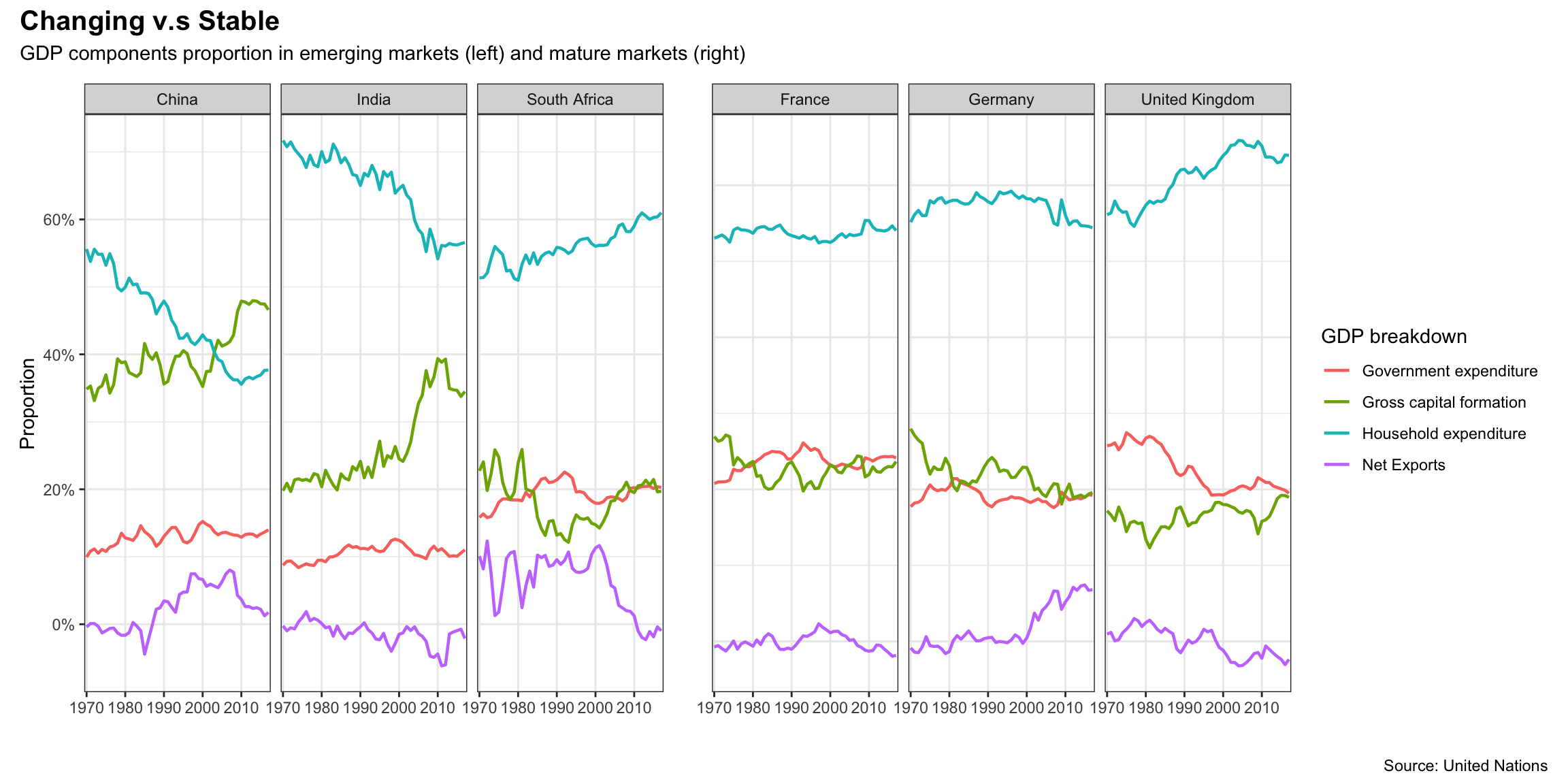
Graph above shows a visible difference between emerging and mature markets. Countries on the left (emerging markets) generally experience more significant variations in GDP structure in comparison with countries on the right (mature markets). The overall higher percentage of government expenditure on the right could be related to the general higher living standards in mature markets.

Both China and India have witnessed growing proportion of Gross Capital Formation and decreasing Household Expenditure during this period. This indicates that investment has been an important booster for GDP growth and could be explained by their ample workforce and favoring policy for investments. In China, Gross Capital Formation grew rapidly between 2000 and 2010, and makes up more in GDP in China than either of the other two countries by the end of given period. This is partly because of continuous investment attracted by China’s opening-up, as well as the return of Hong Kong (1997) and Macau (1999), which gave business investment another boost.

Details

Adapted from: Assignment from Applied Statistics with R, London Business School

Course Instructor: Kostis Christodoulou

Original assignment collaborated with: Study Group 11: Abhinav Bhardwaj, Alberto Lambert, Anna Plaschke, Bartek Makuch, Feiyang Ni