Pay Discrimination Analysis

Background
Are men and women paid differently? In this blog we try to conclude if there is a salary difference between gender in a company called Omega, using predominantly hypothesis testing and bootstrap sampling.
Load the data
As shown below, our data has 3 variables, salary, gender and work experience; and 50 obeservations.
omega <- read_csv(here::here("data", "omega.csv"))
glimpse(omega) # examine the data frame
## Rows: 50
## Columns: 3
## $ salary <dbl> 81894, 69517, 68589, 74881, 65598, 76840, 78800, 70033, 6…
## $ gender <chr> "male", "male", "male", "male", "male", "male", "male", "…
## $ experience <dbl> 16, 25, 15, 33, 16, 19, 32, 34, 1, 44, 7, 14, 33, 19, 24,…Relationship Salary - Gender ?
First, we look at the summary statistics on salary by gender, and create a 95% confidence interval for the mean salary of each gender. The confidence intervals of mean salary are (61486, 67599) and (70088, 76390) for female and male respectively.
But what does is a 95% confidence interval? It means we are 95% confident that the population’s mean salary would be covered by this interval. If we choose our significant level to be 0.05, since there is no overlap between these two confidence intervals, we conclude there is statistically significant difference in salary between male and female employees.
# Summary Statistics of salary by gender
mosaic::favstats (salary ~ gender, data=omega)
## gender min Q1 median Q3 max mean sd n missing
## 1 female 47033 60338 64618 70033 78800 64543 7567 26 0
## 2 male 54768 68331 74675 78568 84576 73239 7463 24 0# Dataframe with two rows (male-female) and having as columns gender, mean, SD, sample size,
# the t-critical value, the standard error, the margin of error,
# and the low/high endpoints of a 95% condifence interval
omega %>%
group_by(gender) %>%
summarise(mean = mean(salary),
SD = sd(salary),
sample_size = n(),
t_critical = qt(0.975, sample_size - 1),
SE = SD/sqrt(sample_size),
margin_of_error = SE*t_critical,
lower_ci = mean - margin_of_error,
upper_ci = mean + margin_of_error)## # A tibble: 2 x 9
## gender mean SD sample_size t_critical SE margin_of_error lower_ci
## <chr> <dbl> <dbl> <int> <dbl> <dbl> <dbl> <dbl>
## 1 female 64543. 7567. 26 2.06 1484. 3056. 61486.
## 2 male 73239. 7463. 24 2.07 1523. 3151. 70088.
## # … with 1 more variable: upper_ci <dbl>We can also use hypothesis testing to see if they are different. Starting with writing down our null and alternative hypothesis:
Null Hypothesis (H0) | Mean salary of male = Mean salary of female in Omega (mean salary of male - mean salary of female = 0)
Alternative Hypothesis (H1) | Mean salary of male != Mean salary of female in Omega (mean salary of male - mean salary of female != 0 in Omega)
Both t test and bootstrap could be used for this question. To give myself more practice, I run both of them and let’s see if they give us the same result.
# hypothesis testing using t.test()
omega <- omega %>%
  mutate(gender = as.factor(gender)) # convert character into factor

t.test(salary ~ gender, data = omega, alternative = 'two.sided')
##
## Welch Two Sample t-test
##
## data: salary by gender
## t = -4, df = 48, p-value = 2e-04
## alternative hypothesis: true difference in means is not equal to 0
## 95 percent confidence interval:
## -12973 -4420
## sample estimates:
## mean in group female mean in group male
## 64543 73239# hypothesis testing using infer package
set.seed(1234)
hypothesis_infer <- omega %>%
specify(salary ~ gender) %>%
hypothesise('independence') %>%
generate(reps = 1000, type = 'permute') %>%
calculate(stat = 'diff in means', order = c('female','male'))
hypothesis_infer %>% get_pvalue(obs_stat = mean(omega$salary[omega$gender == 'female'] ) -
mean(omega$salary[omega$gender == 'male']),
direction = 'both')## # A tibble: 1 x 1
## p_value
## <dbl>
## 1 0In both t.test and bootstrap hypothesis test, the p-value generated is less than the alpha value of 0,05. Therefore, we reject H0 and conclude that there is a statistically significant difference in salary between male and female employees in Omega. Note that in bootstrap, the p-value = 0 is due to rounding, the true value should be really close to 0 but not identical to it.
Relationship Experience - Gender?
(1) - Based on this evidence, can you conclude that there is a significant difference between the experience of the male and female executives? Perform similar analyses as in the previous section. Does your conclusion validate or endanger your conclusion about the difference in male and female salaries?
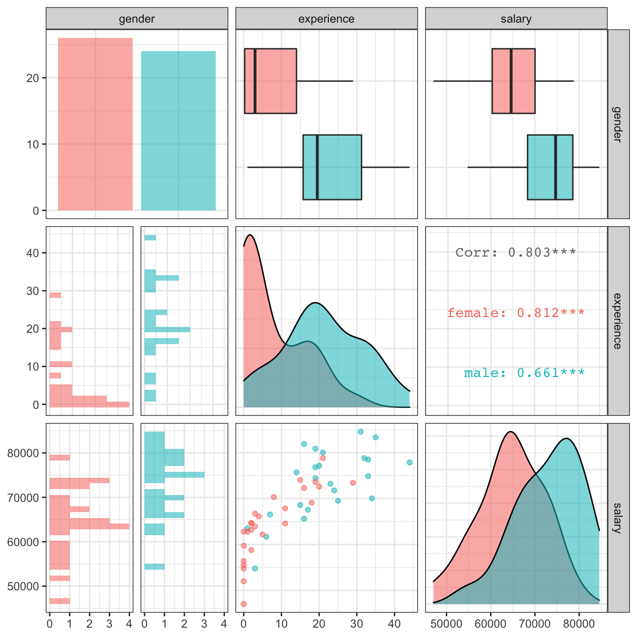
However, if we also look at the boxplot of work experience by gender, we can see women in Omega have less experience than men on average. It could be that the work experience is also affecting men and women’s earning.
omega %>%
  select(gender, experience, salary) %>% #order variables they will appear in ggpairs()
  ggpairs(aes(colour=gender, alpha = 0.3))+
  theme_bw()
To test if there is difference in work experience between men and women in Omega, we run hypothesis testing again:
Null Hypothesis (H0) | Mean work experience of male = Mean work experience of female in Omega (mean work experience of male - mean work experience of female = 0 in Omega)
Alternative Hypothesis (H1) | Mean work experience of male != Mean work experience of female in Omega (mean work experience of male - mean work experience of female != 0 in Omega)
omega %>%
  group_by(gender) %>%
  summarise(mean = mean(experience),
            SD = sd(experience),
            sample_size = n(),
            t_critical = qt(0.975, sample_size - 1),
            SE = SD/sqrt(sample_size),
            margin_of_error = SE*t_critical,
            lower_ci = mean - margin_of_error,
            upper_ci = mean + margin_of_error)
## # A tibble: 2 x 9
## gender mean SD sample_size t_critical SE margin_of_error lower_ci
## <fct> <dbl> <dbl> <int> <dbl> <dbl> <dbl> <dbl>
## 1 female 7.38 8.51 26 2.06 1.67 3.44 3.95
## 2 male 21.1 10.9 24 2.07 2.23 4.61 16.5
## # … with 1 more variable: upper_ci <dbl># hypothesis testing using t.test()
t.test(experience ~ gender, data = omega, alternative = 'two.sided') ##
## Welch Two Sample t-test
##
## data: experience by gender
## t = -5, df = 43, p-value = 1e-05
## alternative hypothesis: true difference in means is not equal to 0
## 95 percent confidence interval:
## -19.35 -8.13
## sample estimates:
## mean in group female mean in group male
## 7.38 21.12# hypothesis testing using infer package
set.seed(1234)
hypothesis_infer <- omega %>%
specify(experience ~ gender) %>%
hypothesise('independence') %>%
generate(reps = 1000, type = 'permute') %>%
calculate(stat = 'diff in means', order = c('female','male'))
hypothesis_infer %>% get_pvalue(obs_stat = mean(omega$experience[omega$gender == 'female'] ) -
mean(omega$experience[omega$gender == 'male']), direction = 'both')## # A tibble: 1 x 1
## p_value
## <dbl>
## 1 0Since there is no overlap in confidence intervals and our p-value is less than the alpha value (a=0.05), we should reject the null hypothesis that the mean work experience of a male employee is equal to the mean work experience of a female employee at Omega. Thus, we can conclude that there is a statistically significant difference in male and female employees’ levels of work experience. This endangers our previous conclusion that the salary difference is because of gender.
Relationship Salary - Experience ?
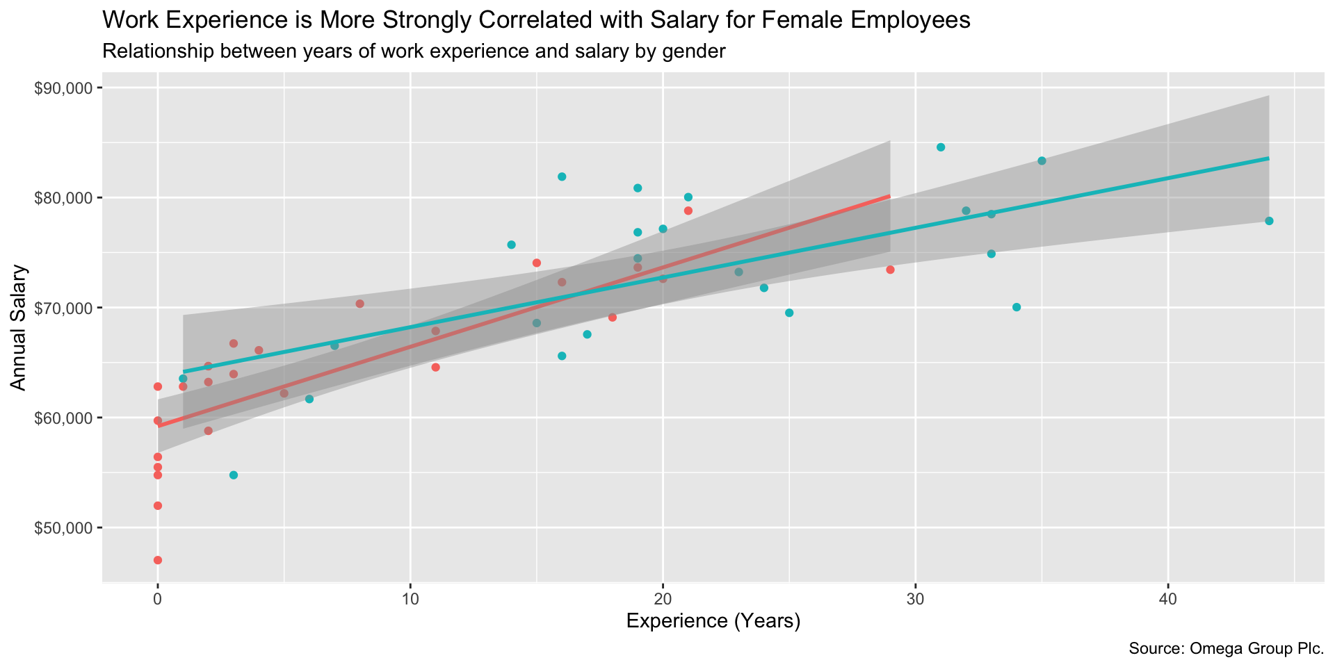
Aha! So it could be possible that the seemingly discrimination in salary between male and female is related to the work experience factor. Let’s use a scatterplot and 2 regression lines to see the relationship between salary and experience.
We can see that in fact, a unit increase in experience is associated with a greater salary increase for female than male employees, since the regression line for female employees is steeper. All the above findings suggest that the salary heterogeneity between female and male employees is a mixed effect of gender, experience and potentially, other (unobserved) variables.
omega %>%
  ggplot(aes(x = experience, y = salary, color = gender)) +
  geom_point() +
  geom_smooth(method = lm, aes(color = gender)) +
  labs(title = 'Work Experience is More Strongly Correlated with Salary for Female Employees',
       subtitle = 'Relationship between years of work experience and salary by gender',
       x = 'Experience (Years)',
       y = 'Annual Salary',
       caption = 'Source: Omega Group Plc.') + theme(legend.position="none") + scale_y_continuous(labels = scales::dollar)
So what is our conclusion? Does gender lead to salary difference? We don’t know the answer. All the tests and regressions we have done show only the association between variables, but not causal effects. However, we can still use gender, work experience and other features of an employee to predict or explain their salary.
Details
Adapted from: Assignment from Applied Statistics with R, London Business School
Course Instructor: Kostis Christodoulou
Original assignment collaborated with: Study Group 11: Abhinav Bhardwaj, Alberto Lambert, Anna Plaschke, Bartek Makuch, Feiyang Ni